Prim's algorithm
| Graph and tree search algorithms |
|---|
| Listings |
|
| Related topics |
In computer science, Prim's algorithm is a greedy algorithm that finds a minimum spanning tree for a weighted undirected graph. This means it finds a subset of the edges that forms a tree that includes every vertex, where the total weight of all the edges in the tree is minimized. The algorithm operates by building this tree one vertex at a time, from an arbitrary starting vertex, at each step adding the cheapest possible connection from the tree to another vertex.
The algorithm was developed in 1930 by Czech mathematician Vojtěch Jarník[1] and later rediscovered and republished by computer scientists Robert C. Prim in 1957[2] and Edsger W. Dijkstra in 1959.[3] Therefore, it is also sometimes called the DJP algorithm,[4] Jarník's algorithm,[5] the Prim–Jarník algorithm,[6] or the Prim–Dijkstra algorithm.[7]
Other well-known algorithms for this problem include Kruskal's algorithm and Borůvka's algorithm.[8] These algorithms find the minimum spanning forest in a possibly disconnected graph; in contrast, the most basic form of Prim's algorithm only finds minimum spanning trees in connected graphs. However, running Prim's algorithm separately for each connected component of the graph, it can also be used to find the minimum spanning forest.[9] In terms of their asymptotic time complexity, these three algorithms are equally fast for sparse graphs, but slower than other more sophisticated algorithms.[4][7] However, for graphs that are sufficiently dense, Prim's algorithm can be made to run in linear time, meeting or improving the time bounds for other algorithms.[10]

Description
The algorithm may informally be described as performing the following steps:
- Initialize a tree with a single vertex, chosen arbitrarily from the graph.
- Grow the tree by one edge: of the edges that connect the tree to vertices not yet in the tree, find the minimum-weight edge, and transfer it to the tree.
- Repeat step 2 (until all vertices are in the tree).
In more detail, it may be implemented following the pseudocode below.
- Associate with each vertex v of the graph a number C[v] (the cheapest cost of a connection to v) and an edge E[v] (the edge providing that cheapest connection). To initialize these values, set all values of C[v] to +∞ (or to any number larger than the maximum edge weight) and set each E[v] to a special flag value indicating that there is no edge connecting v to earlier vertices.
- Initialize an empty forest F and a set Q of vertices that have not yet been included in F (initially, all vertices).
- Repeat the following steps until Q is empty:
- Find and remove a vertex v from Q having the minimum possible value of C[v]
- Add v to F and, if E[v] is not the special flag value, also add E[v] to F
- Loop over the edges vw connecting v to other vertices w. For each such edge, if w still belongs to Q and vw has smaller weight than C[w], perform the following steps:
- Set C[w] to the cost of edge vw
- Set E[w] to point to edge vw.
- Return F
As described above, the starting vertex for the algorithm will be chosen arbitrarily, because the first iteration of the main loop of the algorithm will have a set of vertices in Q that all have equal weights, and the algorithm will automatically start a new tree in F when it completes a spanning tree of each connected component of the input graph. The algorithm may be modified to start with any particular vertex s by setting C[s] to be a number smaller than the other values of C (for instance, zero), and it may be modified to only find a single spanning tree rather than an entire spanning forest (matching more closely the informal description) by stopping whenever it encounters another vertex flagged as having no associated edge.
Different variations of the algorithm differ from each other in how the set Q is implemented: as a simple linked list or array of vertices, or as a more complicated priority queue data structure. This choice leads to differences in the time complexity of the algorithm. In general, a priority queue will be quicker at finding the vertex v with minimum cost, but will entail more expensive updates when the value of C[w] changes.
Time complexity

The time complexity of Prim's algorithm depends on the data structures used for the graph and for ordering the edges by weight, which can be done using a priority queue. The following table shows the typical choices:
| Minimum edge weight data structure | Time complexity (total) |
|---|---|
| adjacency matrix, searching | |
| binary heap and adjacency list | |
| Fibonacci heap and adjacency list |
A simple implementation of Prim's, using an adjacency matrix or an adjacency list graph representation and linearly searching an array of weights to find the minimum weight edge, to add requires O(|V|2) running time. However, this running time can be greatly improved further by using heaps to implement finding minimum weight edges in the algorithm's inner loop.
A first improved version uses a heap to store all edges of the input graph, ordered by their weight. This leads to an O(|E| log |E|) worst-case running time. But storing vertices instead of edges can improve it still further. The heap should order the vertices by the smallest edge-weight that connects them to any vertex in the partially constructed minimum spanning tree (MST) (or infinity if no such edge exists). Every time a vertex v is chosen and added to the MST, a decrease-key operation is performed on all vertices w outside the partial MST such that v is connected to w, setting the key to the minimum of its previous value and the edge cost of (v,w).
Using a simple binary heap data structure, Prim's algorithm can now be shown to run in time O(|E| log |V|) where |E| is the number of edges and |V| is the number of vertices. Using a more sophisticated Fibonacci heap, this can be brought down to O(|E| + |V| log |V|), which is asymptotically faster when the graph is dense enough that |E| is ω(|V|), and linear time when |E| is at least |V| log |V|. For graphs of even greater density (having at least |V|c edges for some c > 1), Prim's algorithm can be made to run in linear time even more simply, by using a d-ary heap in place of a Fibonacci heap.[10][11]

Proof of correctness
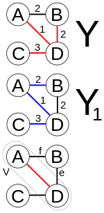
Let P be a connected, weighted graph. At every iteration of Prim's algorithm, an edge must be found that connects a vertex in a subgraph to a vertex outside the subgraph. Since P is connected, there will always be a path to every vertex. The output Y of Prim's algorithm is a tree, because the edge and vertex added to tree Y are connected. Let Y1 be a minimum spanning tree of graph P. If Y1=Y then Y is a minimum spanning tree. Otherwise, let e be the first edge added during the construction of tree Y that is not in tree Y1, and V be the set of vertices connected by the edges added before edge e. Then one endpoint of edge e is in set V and the other is not. Since tree Y1 is a spanning tree of graph P, there is a path in tree Y1 joining the two endpoints. As one travels along the path, one must encounter an edge f joining a vertex in set V to one that is not in set V. Now, at the iteration when edge e was added to tree Y, edge f could also have been added and it would be added instead of edge e if its weight was less than e, and since edge f was not added, we conclude that
Let tree Y2 be the graph obtained by removing edge f from and adding edge e to tree Y1. It is easy to show that tree Y2 is connected, has the same number of edges as tree Y1, and the total weights of its edges is not larger than that of tree Y1, therefore it is also a minimum spanning tree of graph P and it contains edge e and all the edges added before it during the construction of set V. Repeat the steps above and we will eventually obtain a minimum spanning tree of graph P that is identical to tree Y. This shows Y is a minimum spanning tree.
See also
- Dijkstra's algorithm, a very similar algorithm for the shortest path problem
References
- ↑ Jarník, V. (1930), "O jistém problému minimálním" [About a certain minimal problem], Práce Moravské Přírodovědecké Společnosti (in Czech), 6: 57–63.
- ↑ Prim, R. C. (November 1957), "Shortest connection networks And some generalizations", Bell System Technical Journal, 36 (6): 1389–1401, doi:10.1002/j.1538-7305.1957.tb01515.x.
- ↑ Dijkstra, E. W. (1959), "A note on two problems in connexion with graphs" (PDF), Numerische Mathematik, 1: 269–271, doi:10.1007/BF01386390.
- 1 2 Pettie, Seth; Ramachandran, Vijaya (2002), "An optimal minimum spanning tree algorithm", Journal of the ACM, 49 (1): 16–34, doi:10.1145/505241.505243, MR 2148431.
- ↑ Sedgewick, Robert; Wayne, Kevin Daniel (2011), Algorithms (4th ed.), Addison-Wesley, p. 628, ISBN 9780321573513.
- ↑ Rosen, Kenneth (2011), Discrete Mathematics and Its Applications (7th ed.), McGraw-Hill Science, p. 798.
- 1 2 Cheriton, David; Tarjan, Robert Endre (1976), "Finding minimum spanning trees", SIAM Journal on Computing, 5 (4): 724–742, doi:10.1137/0205051, MR 0446458.
- ↑ Tarjan, Robert Endre (1983), "Chapter 6. Minimum spanning trees. 6.2. Three classical algorithms", Data Structures and Network Algorithms, CBMS-NSF Regional Conference Series in Applied Mathematics, 44, Society for Industrial and Applied Mathematics, pp. 72–77.
- ↑ Kepner, Jeremy; Gilbert, John (2011), Graph Algorithms in the Language of Linear Algebra, Software, Environments, and Tools, 22, Society for Industrial and Applied Mathematics, p. 55, ISBN 9780898719901.
- 1 2 Tarjan (1983), p. 77.
- ↑ Johnson, Donald B. (December 1975), "Priority queues with update and finding minimum spanning trees", Information Processing Letters, 4 (3): 53–57, doi:10.1016/0020-0190(75)90001-0.
External links
- Prim's Algorithm with example and program in c
 Media related to Prim's Algorithm at Wikimedia Commons