Partial equilibrium
| Economics |
|---|
_Per_Capita_in_2015.svg.png) |
|
|
| By application |
|
| Lists |
|
Partial equilibrium is a condition of economic equilibrium which takes into consideration only a part of the market, ceteris paribus, to attain equilibrium.
As defined by George Stigler, "A partial equilibrium is one which is based on only a restricted range of data, a standard example is price of a single product, the prices of all other products being held fixed during the analysis."[1]
The supply and demand model is a partial equilibrium model where the clearance on the market of some specific goods is obtained independently from prices and quantities in other markets. In other words, the prices of all substitutes and complements, as well as income levels of consumers, are taken as given. This makes analysis much simpler than in a general equilibrium model which includes an entire economy.
Here the dynamic process is that prices adjust until supply equals demand. It is a powerfully simple technique that allows one to study equilibrium, efficiency and comparative statics. The stringency of the simplifying assumptions inherent in this approach make the model considerably more tractable, but may produce results which, while seemingly precise, do not effectively model real-world economic phenomena.
Partial equilibrium analysis examines the effects of policy action in creating equilibrium only in that particular sector or market which is directly affected, ignoring its effect in any other market or industry assuming that they being small will have little impact if any.
Hence this analysis is considered to be useful in constricted markets.
Léon Walras first formalized the idea of a one-period economic equilibrium of the general economic system, but it was French economist Antoine Augustin Cournot and English political economist Alfred Marshall who developed tractable models to analyze an economic system.
Assumptions
- Commodity price is given and constant for the consumers.
- Consumers' taste and preferences, habits, incomes are also considered to be constant.
- Prices of prolific resources of a commodity and that of other related goods (substitute or complementary) are known as well as constant.
- Industry is easily availed with factors of production at a known and constant price compliant with the methods of production in use.
- Prices of the products that the factor of production helps in producing and the price and quantity of other factors are known and constant.
- There is perfect mobility of factors of production between occupation and places.
The above-mentioned points relate to a perfectly competitive market but can be further extended to monopolistic competition, oligopoly, monopoly and monopsony markets.[2]
Applications
Applications of partial equilibrium discusses, when does an individual, a firm, an industry, factors of production attain their equilibrium points-
- A consumer is in a state of equilibrium when they achieve maximum aggregate satisfaction on the expenditure that they make depending on the set of conditions relating to his tastes and preferences, income, price and supply of the commodity etc.
- Producers’ equilibrium occurs when they maximize their net profit subject to a given set of economic situations.
- A firm's equilibrium point is when it has no inclination in changing its production.
- In the short run: Marginal Revenue = Marginal Cost.
Algebraically MR=MC
- In long run: Long run Marginal Cost = Marginal Revenue = Average Revenue = Long run Average Cost
Algebraically LMC=MR=AR=LAC at its minimum are the conditions of equilibrium.[3] It means that a firm is earning only a "normal profit" and has no intension to leave the industry.
- Equilibrium for an industry happens when there is normal profit made by an industry It is such a situation when no new firm wants to enter into it and the existing firm does not want to exit.
Only one price prevails in the market for a single product where the quantity of goods purchased by a buyer = total quantity produced by different firms. All the firms produces till that level where Marginal Cost=Marginal Revenue, and sells the product at market price ruling at that point of time.[4]
- Factors of production, i.e., land, labor, capital, and entrepreneurs are in equilibrium when they are paid the maximum possible so as maximize the income. Here the Price = Marginal Revenue Product.
At this price it does not have any enticement to look for employment anywhere else.
The quantity of factors which its owners want to sell should be equal to the quantity which the entrepreneurs are ready to hire.
Limitations
- It is restricted to one particular portion of the economy.
- It lacks the ability to study the interrelations of all the parts of the economy.
- This analysis will fail if the improbable assumptions, which disconnect the study of specific market from the rest of the economy, are not taken into consideration.
- It has been unsuccessful in explaining the outcome of economic disturbance in the market that leads to demand and supply changes, moving from one market to another and thus instigating second- and third-order waves of change in the whole economy.
Welfare effect of trade policies


In partial equilibrium the welfare effects on consumers who purchase and the producers who produce in the market is distinguished by consumer surplus and producer surplus.
Consumer surplus
The amount that a consumer is ready to pay for a particular good minus the amount that the consumer actually pays. The amount that the consumer is willing to pay has to be greater.[5]
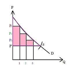
In the graph given here, P1 is the price that a consumer is ready to pay for a particular product. But the producer may reduce the price to P2 expecting that either more people would buy at the reduced rate, or the person who was ready to pay P1 will purchase more of the same. The producer may further reduce the price to P3, again expecting more buyers or the same buyers purchasing more.[5]
The price keeps on falling until P’, where the demand and the supply curves intersect: their intersection is the equilibrium point. Hence the consumer surplus for first consumer can be calculated as P1 - P’, decreasing for the second consumer to P2 - P’, and so on. Thus the total consumer surplus in the market can be obtained by summing up the three rectangles. The triangle with the purple outline to the left indicates that area.[5]
Producer surplus
Amount that a producer finally receives by selling a particular product minus the amount the producer is ready to accept for that good. The amount that the producer receives should be greater.[5]
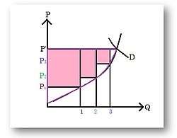
If only one unit of the commodity was demanded at the price P1, this becomes the price which the producer expects to receive. But if two units are demanded, the minimum price at which the producer would be ready to increase the supply shifts to P2. This continues and the final price that ultimately prevails in the market is P’, the price which is obtained by the intersection of the demand and supply curve in the market. The producer's surplus here would be initial price minus the final price. And total consumer surplus in the market will be summation of the three rectangles.[5]
Difference between Partial and General Equilibrium
| Partial Equilibrium | General Equilibrium |
|---|---|
| • Developed by Alfred Marshall.[6] | • Léon Walras was first to develop it. |
| • Related to single variable | • More than one variable or economy as a whole is taken into consideration |
• Based on two assumptions:
|
• It is based on the assumption that various sectors are mutually interdependent.
There is an effect on other sectors due to change in one. |
| • Other things remaining constant, price of a good is determined | •Prices of goods are determined simultaneously and mutually.
Hence all product and factor markets are simultaneously in equilibrium. |
See also
References
- ↑ Jain, T.R. (2006-07). Microeconomics and Basic Mathematics. New Delhi: VK Publications. p. 28. ISBN 81-87140-89-5. Check date values in:
|date=(help) - ↑ Jhingan, M.L (6th edition). Microeconomic Theory. Vrinda Publications. p. 130. ISBN 81-8281-071-X. Check date values in:
|date=(help) - ↑ Mandal, Ram Krishna (2007). Microeconomic Theory. Atlantic Publishers & Dist. p. 313.
- ↑ "Eqilibrium". Retrieved 4 October 2011.
- 1 2 3 4 5 6 7 Suranovic, Steve (2004). International Trade Theory And Policy. ISBN 978-1-936126-44-6.
- ↑ "Economics Online". Retrieved 4 October 2011.