Multifractal system

A Strange Attractor that exhibits multifractal scaling

Example of a multifractal electronic eigenstate at the Anderson localization transition in a system with 1367631 atoms.

A multifractal system is a generalization of a fractal system in which a single exponent (the fractal dimension) is not enough to describe its dynamics; instead, a continuous spectrum of exponents (the so-called singularity spectrum) is needed.^[1]

Multifractal systems are common in nature, especially geophysics. They include the length of coastlines, fully developed turbulence, stock market time series, real world scenes, the Sun’s magnetic field time series, heartbeat dynamics, human gait, and natural luminosity time series. Models have been proposed in various contexts ranging from turbulence in fluid dynamics to internet traffic, finance, image modeling, texture synthesis, meteorology, geophysics and more. The origin of multifractality in sequential (time series) data has been attributed to mathematical convergence effects related to the central limit theorem that have as foci of convergence the family of statistical distributions known as the Tweedie exponential dispersion models^[2] as well as the geometric Tweedie models.^[3] The first convergence effect yields monofractal sequences and the second convergence effect is responsible for variation in the fractal dimension of the monofractal sequences.^[4]

From a practical perspective, multifractal analysis uses the mathematical basis of multifractal theory to investigate datasets, often in conjunction with other methods of fractal analysis and lacunarity analysis. The technique entails distorting datasets extracted from patterns to generate multifractal spectra that illustrate how scaling varies over the dataset. The techniques of multifractal analysis have been applied in a variety of practical situations such as predicting earthquakes and interpreting medical images.^[5]^[6]^[7]

Definition

In a multifractal system $s$ , the behavior around any point is described by a local power law:

s({\vec {x}}+{\vec {a}})-s({\vec {x}})\sim a^{h({\vec {x}})}.

The exponent $h({\vec {x}})$ is called the singularity exponent, as it describes the local degree of singularity or regularity around the point ${\vec {x}}$ .

The ensemble formed by all the points that share the same singularity exponent is called the singularity manifold of exponent h, and is a fractal set of fractal dimension D(h). The curve D(h) versus h is called the singularity spectrum and fully describes the (statistical) distribution of the variable $s$ .

In practice, the multifractal behaviour of a physical system $X$ is not directly characterized by its singularity spectrum D(h). Data analysis rather gives access to the multiscaling exponents $\zeta (q),\ q\in {\mathbb {R} }$ . Indeed, multifractal signals generally obey a scale invariance property which yields power law behaviours for multiresolution quantities depending on their scale $a$ . Depending on the object under study, these multiresolution quantities, denoted by $T_{X}(a)$ in the following, can be local averages in boxes of size $a$ , gradients over distance $a$ , wavelet coefficients at scale $a$ ... For multifractal objects, one usually observes a global power law scaling of the form:

\langle T_{X}(a)^{q}\rangle \sim a^{\zeta (q)}\

at least in some range of scales and for some range of orders $q$ . When such a behaviour is observed, one talks of scale invariance, self-similarity or multiscaling.^[8]

Estimation

Using the so-called multifractal formalism, it can be shown that, under some well-suited assumptions, there exists a correspondence between the singularity spectrum $D(h)$ and the multiscaling exponents $\zeta (q)$ through a Legendre transform. While the determination of $D(h)$ calls for some exhaustive local analysis of the data, which would result in difficult and numerically unstable calculations, the estimation of the $\zeta (q)$ relies on the use of statistical averages and linear regressions in log-log diagrams. Once the $\zeta (q)$ are known, one can deduce an estimate of $D(h)$ thanks to a simple Legendre transform.

Multifractal systems are often modeled by stochastic processes such as multiplicative cascades. Interestingly, the $\zeta (q)$ receives some statistical interpretation as they characterize the evolution of the distributions of the $T_{X}(a)$ as $a$ goes from larger to smaller scales. This evolution is often called statistical intermittency and betrays a departure from Gaussian models.

Modelling as a multiplicative cascade also leads to estimation of multifractal properties (Roberts & Cronin 1996). This methods works reasonably well even for relatively small datasets A maximum likelihood fit of a multiplicative cascade to the dataset not only estimates the complete spectrum, but also gives reasonable estimates of the errors (see the web service ).

Practical application of multifractal spectra

Multifractal analysis is analogous to viewing a dataset through a series of distorting lenses to home in on differences in scaling. The pattern shown is a Hénon map

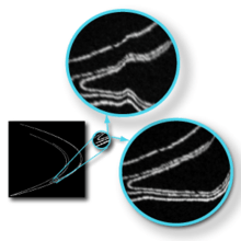
Multifractal analysis has been used in several fields in science to characterize various types of datasets.^[9] In essence, multifractal analysis applies a distorting factor to datasets extracted from patterns, to compare how the data behave at each distortion. This is done using graphs known as multifractal spectra that illustrate how the distortions affect the data, analogous to viewing the dataset through a "distorting lens" as shown in the illustration.^[10] Several types of multifractal spectra are used in practise.

D_Q vs Q

D_Q vs Q spectra for a non-fractal circle (empirical box counting dimension = 1.0), mono-fractal Quadric Cross (empirical box counting dimension = 1.49), and multifractal Hénon map (empirical box counting dimension = 1.29).

One practical multifractal spectrum is the graph of D_Q vs Q, where D_Q is the generalized dimension for a dataset and Q is an arbitrary set of exponents. The expression generalized dimension thus refers to a set of dimensions for a dataset (detailed calculations for determining the generalized dimension using box counting are described below).

Dimensional ordering

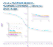
The general pattern of the graph of D_Q vs Q can be used to assess the scaling in a pattern. The graph is generally decreasing, sigmoidal around Q=0, where D_(Q=0) ≥ D_(Q=1) ≥ D_(Q=2). As illustrated in the figure, variation in this graphical spectrum can help distinguish patterns. The image shows D_(Q) spectra from a multifractal analysis of binary images of non-, mono-, and multi-fractal sets. As is the case in the sample images, non- and mono-fractals tend to have flatter D_(Q) spectra than multifractals.

The generalized dimension also offers some important specific information. D_(Q=0) is equal to the capacity dimension, which in the analysis shown in the figures here is the box counting dimension. D_(Q=1) is equal to the information dimension, and D_(Q=2) to the correlation dimension. This relates to the "multi" in multifractal whereby multifractals have multiple dimensions in the D_(Q) vs Q spectra but monofractals stay rather flat in that area.^[10]^[11]

$f(\alpha )$ vs $\alpha$

Another useful multifractal spectrum is the graph of $f(\alpha )$ vs $\alpha$ (see calculations). These graphs generally rise to a maximum that approximates the fractal dimension at Q=0, and then fall. Like D_Q vs Q spectra, they also show typical patterns useful for comparing non-, mono-, and multi-fractal patterns. In particular, for these spectra, non- and mono-fractals converge on certain values, whereas the spectra from multifractal patterns are typically humped over a broader extent.

Generalized dimensions of species abundance distributions in space

One application of D_q vs q in ecology is the characterization of the abundance distribution of species. Traditionally the relative species abundances is calculated for an area of study without taken into account the positions of the individuals. An equivalent representation of relative species abundances are species ranks ^[12] and this can be used to generate a surface called the species-rank surface^[12] which can be analyzed using generalized dimensions to detect different ecological mechanisms like the ones observed in neutral theory of biodiversity , metacommunity dynamics or niche theory.^[12]^[13]

Estimating multifractal scaling from box counting

Multifractal spectra can be determined from box counting on digital images. First, a box counting scan is done to determine how the pixels are distributed; then, this "mass distribution" becomes the basis for a series of calculations.^[10]^[11]^[14] The chief idea is that for multifractals, the probability, $P$ , of a number of pixels, $m$ , appearing in a box, $i$ , varies as box size, $\epsilon$ , to some exponent, $\alpha$ , which changes over the image, as in Eq.0.0. NB: For monofractals, in contrast, the exponent does not change meaningfully over the set. $P$ is calculated from the box counting pixel distribution as in Eq.2.0.

$P_{[i,\epsilon ]}\varpropto \epsilon ^{-\alpha _{i}}\therefore \alpha _{i}\varpropto {\frac {\log {P_{[i,\epsilon ]}}}{\log {\epsilon ^{-1}}}}$

(Eq.0.0)

\epsilon

= an arbitrary scale (box size in box counting) at which the set is examined

i

= the index for each box laid over the set for an

\epsilon

m_{[i,\epsilon ]}

= the number of pixels or mass in any box,

i

, at size

\epsilon

N_{\epsilon }

= the total boxes that contained more than 0 pixels, for each

\epsilon

$M_{\epsilon }=\sum _{i=1}^{N_{\epsilon }}m_{[i,\epsilon ]}=$ the total mass or sum of pixels in all boxes for this $\epsilon$

(Eq.1.0)

$P_{[i,\epsilon ]}={\frac {m_{[i,\epsilon ]}}{M_{\epsilon }}}=$ the probability of this mass at $i$ relative to the total mass for a box size

(Eq.2.0)

$P$ is used to observe how the pixel distribution behaves when distorted in certain ways as in Eq.3.0 and Eq.3.1:

Q

= an arbitrary range of values to use as exponents for distorting the data set

$I_{{(Q)}_{[\epsilon ]}}=\sum _{i=1}^{N_{\epsilon }}{P_{[i,\epsilon ]}^{Q}}=$ the sum of all mass probabilities distorted by being raised to this Q, for this box size

(Eq.3.0)

When $Q=1$ , Eq.3.0 equals 1, the usual sum of all probabilities, and when $Q=0$ , every term is equal to 1, so the sum is equal to the number of boxes counted, $N_{\epsilon }$ .

$\mu _{{(Q)}_{[i,\epsilon ]}}={\frac {P_{[i,\epsilon ]}^{Q}}{I_{{(Q)}_{[\epsilon ]}}}}=$ how the distorted mass probability at a box compares to the distorted sum over all boxes at this box size

(Eq.3.1)

These distorting equations are further used to address how the set behaves when scaled or resolved or cut up into a series of $\epsilon$ -sized pieces and distorted by Q, to find different values for the dimension of the set, as in the following:

An important feature of Eq.3.0 is that it can also be seen to vary according to scale raised to the exponent $\tau$ in Eq.4.0:

$I_{{(Q)}_{[\epsilon ]}}\varpropto \epsilon ^{\tau _{(Q)}}$

(Eq.4.0)

Thus, a series of values for $\tau _{(Q)}$ can be found from the slopes of the regression line for the log of Eq.3.0 versus the log of $\epsilon$ for each $Q$ , based on Eq.4.1:

$\tau _{(Q)}={\lim _{\epsilon \to 0}{\left[{\frac {\log {I_{{(Q)}_{[\epsilon ]}}}}{\log {\epsilon }}}\right]}}$

(Eq.4.1)

For the generalized dimension:

$D_{(Q)}={\lim _{\epsilon \to 0}{\left[{\frac {\log {I_{{(Q)}_{[\epsilon ]}}}}{\log {\epsilon ^{-1}}}}\right]}}{(1-Q)^{-1}}$

(Eq.5.0)

$D_{(Q)}={\frac {\tau _{(Q)}}{Q-1}}$

(Eq.5.1)

$\tau _{{(Q)}_{}}=D_{(Q)}\left(Q-1\right)$

(Eq.5.2)

$\tau _{(Q)}=\alpha _{(Q)}Q-f_{\left(\alpha _{(Q)}\right)}$

(Eq.5.3)

$\alpha _{(Q)}$ is estimated as the slope of the regression line for $\epsilon$ versus $\epsilon$ where:

$A_{\epsilon ,Q}=\sum _{i=1}^{N_{\epsilon }}{\mu _{{i,\epsilon }_{Q}}{P_{{i,\epsilon }_{Q}}}}$

(Eq.6.0)

Then $f_{\left(\alpha _{(Q)}\right)}$ is found from Eq.5.3.

The mean $\tau _{(Q)}$ is estimated as the slope of the log-log regression line for $\tau _{{(Q)}_{[\epsilon ]}}$ versus $\epsilon$ , where:

$\tau _{(Q)_{[\epsilon ]}}={\frac {\sum _{i=1}^{N_{\epsilon }}{P_{[i,\epsilon ]}^{Q-1}}}{N_{\epsilon }}}$

(Eq.6.1)

In practise, the probability distribution depends on how the dataset is sampled, so optimizing algorithms have been developed to ensure adequate sampling.^[10]

References

↑ Harte, David (2001). Multifractals. London: Chapman & Hall. ISBN 978-1-58488-154-4.
↑ Kendal, WS; Jørgensen, BR (2011). "Tweedie convergence: a mathematical basis for Taylor's power law, 1/f noise and multifractality". Phys. Rev E. 84: 066120. doi:10.1103/physreve.84.066120.
↑ Jørgensen, B; Kokonendji, CC (2011). "Dispersion models for geometric sums". Braz J Probab Stat. 25: 263–293. doi:10.1214/10-bjps136.
↑ Kendal, WS (2014). "Multifractality attributed to dual central limit-like convergence effects". Physica A. 401: 22–33. doi:10.1016/j.physa.2014.01.022.
↑ Lopes, R.; Betrouni, N. (2009). "Fractal and multifractal analysis: A review". Medical Image Analysis. 13 (4): 634–649. doi:10.1016/j.media.2009.05.003. PMID 19535282.
↑ Moreno, P. A.; Vélez, P. E.; Martínez, E.; Garreta, L. E.; Díaz, N. S.; Amador, S.; Tischer, I.; Gutiérrez, J. M.; Naik, A. K.; Tobar, F. N.; García, F. (2011). "The human genome: A multifractal analysis". BMC Genomics. 12: 506. doi:10.1186/1471-2164-12-506. PMC 3277318. PMID 21999602.
↑ Atupelage, C.; Nagahashi, H.; Yamaguchi, M.; Sakamoto, M.; Hashiguchi, A. (2012). "Multifractal feature descriptor for histopathology". Analytical Cellular Pathology. 35 (2): 123–126. doi:10.3233/ACP-2011-0045. PMID 22101185.
↑ A.J. Roberts and A. Cronin (1996). "Unbiased estimation of multi-fractal dimensions of finite data sets". Physica A. 233: 867–878. doi:10.1016/S0378-4371(96)00165-3.
↑ Trevino, J.; Liew, S. F.; Noh, H.; Cao, H.; Dal Negro, L. (2012). "Geometrical structure, multifractal spectra and localized optical modes of aperiodic Vogel spirals". Optics Express. 20 (3): 3015. doi:10.1364/OE.20.003015.
1 2 3 4 Karperien, A (2002), What are Multifractals?, ImageJ, archived from the original on 2012-02-10, retrieved 2012-02-10
1 2 Chhabra, A.; Jensen, R. (1989). "Direct determination of the f(α) singularity spectrum". Physical Review Letters. 62 (12): 1327–1330. Bibcode:1989PhRvL..62.1327C. doi:10.1103/PhysRevLett.62.1327. PMID 10039645.
1 2 3 Saravia, Leonardo A. (2015-08-01). "A new method to analyse species abundances in space using generalized dimensions". Methods in Ecology and Evolution: n/a–n/a. doi:10.1111/2041-210X.12417. ISSN 2041-210X.
↑ Saravia, Leonardo A. (2014-01-01). "mfSBA: Multifractal analysis of spatial patterns in ecological communities". F1000Research. 3: 14. doi:10.12688/f1000research.3-14.v2. PMC 4197745. PMID 25324962.
↑ Posadas, A. N. D.; Giménez, D.; Bittelli, M.; Vaz, C. M. P.; Flury, M. (2001). "Multifractal Characterization of Soil Particle-Size Distributions". Soil Science Society of America Journal. 65 (5): 1361. doi:10.2136/sssaj2001.6551361x.
↑ M. K. Hassan, M. Z. Hassan and N. I. Pavel, “Scale-free network topology and multifractality in a weighted planar stochastic lattice” New Journal of Physics 12 093045 ( 2010) http://doi:10.1088/1367-2630/12/9/093045

Veneziano, Daniele; Essiam, Albert K. (June 1, 2003). "Flow through porous media with multifractal hydraulic conductivity". Water Resources Research. 39 (6). Bibcode:2003WRR....39.1166V. doi:10.1029/2001WR001018. ISSN 1944-7973. Retrieved April 15, 2014.

External links

Stanley H.E., Meakin P. (1988). "Multifractal phenomena in physics and chemistry" (Review). Nature. 335 (6189): 405–9. doi:10.1038/335405a0.
Arneodo, Alain; Audit, Benjamin; Kestener, Pierre; Roux, Stephane (2008). "Wavelet-based multifractal analysis". Scholarpedia. 3 (3): 4103. doi:10.4249/scholarpedia.4103. ISSN 1941-6016.
Movies of visualizations of multifractals

Fractals

Characteristics	Fractal dimensions Assouad Box-counting Correlation Hausdorff Packing Topological Recursion Self-similarity

Iterated function system	Barnsley fern Cantor set Dragon curve Koch snowflake Menger sponge Sierpinski carpet Sierpinski triangle Space-filling curve T-square

Strange attractor	Multifractal system

L-system	Space-filling curve

Escape-time fractals	Burning Ship fractal Julia set Filled Lyapunov fractal Mandelbrot set Nova fractal

Random fractals	Brownian motion Brownian tree Diffusion-limited aggregation Fractal landscape Lévy flight Percolation theory Self-avoiding walk

People	Georg Cantor Felix Hausdorff Gaston Julia Helge von Koch Paul Lévy Aleksandr Lyapunov Benoit Mandelbrot Lewis Fry Richardson Wacław Sierpiński

Other	"How Long Is the Coast of Britain?" Coastline paradox List of fractals by Hausdorff dimension The Beauty of Fractals (1986 book)

This article is issued from Wikipedia - version of the 12/3/2016. The text is available under the Creative Commons Attribution/Share Alike but additional terms may apply for the media files.